Automatic Speech Recognition (ASR) From Scratch (With Intuition)

Note 2 — The implementation will assume some basic knowledge about the transformer architecture and CNNs.

The transformer architecture was originally proposed for solving complex tasks in the field of natural language processing. However, since then, it has been applied to other modalities as well, where it has performed significantly better than the predecessors (CNNs, HMMs, GMMs, etc.). That said, we can not just plug in the vanilla transformer architecture and expect it to give SOTA results in all the modalities.

Why Is Speech Significantly More Difficult Than Text?

For starters, in the field of speech, many languages in the world do not even have a written script, so how do we enable a machine to learn a language that can not be represented in discrete, text-based tokens? There are workarounds, but discussing that would need a separate article, so we will not delve into this here.

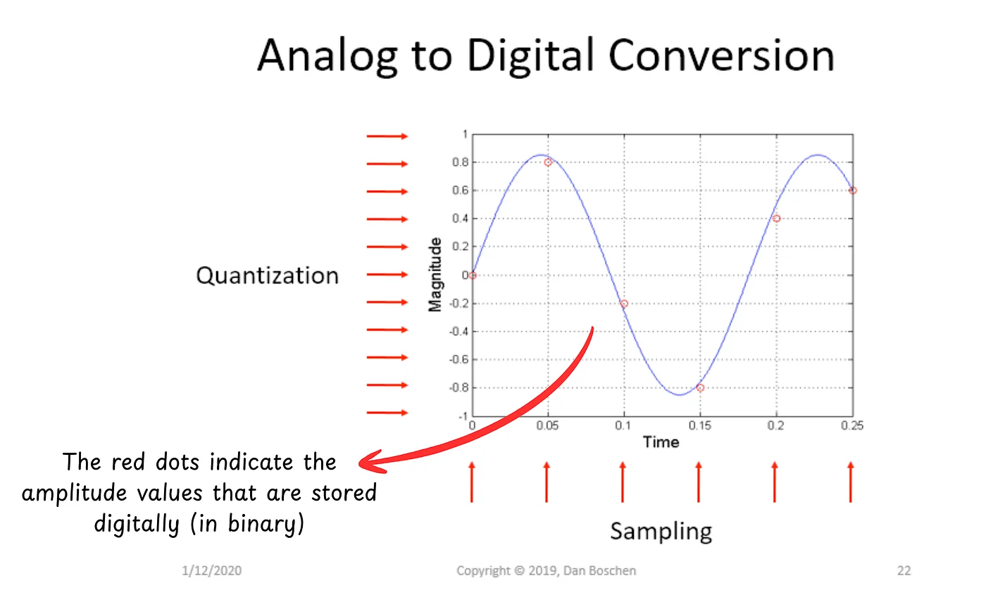Analog-to-digital conversion process for audio signals (Image taken from https://dsp.stackexchange.com/a/63179, annotated by the author)

More importantly, speech is a continuous signal (as compared to text, which is discrete). To convert speech into a digital format, we use something called sampling and quantization. In layman’s terms, sampling rate basically defines the number of amplitude observations per second (so obviously, the higher the sampling rate, the cleaner the audio). Now, the standard sampling rate for digital audio is 44.1 kHz. So, for a 3-second audio, we have,

\[44100 \times 3 = 132300 \text{ amplitude values}\]

In the case of a vanilla transformer with half-precision, this results in an attention matrix of about (132300)² elements (since attention scales quadratically with sequence length), which roughly comes out to be about 32.6 GB worth of VRAM.

Just to scratch that itch of curiosity, this equates to approximately 12.7 TB worth of VRAM for a 1-minute-long digital audio, which is WAY beyond the capabilities of current GPUs, even with distributed training.

This is where feature extraction comes in!

Are All Those Amplitude Values Useful?

In one word, no.

If I reduce the sampling rate from 44.1 kHz to 16 kHz (say), I will still have a speech signal whose semantic meaning stays the same. So, in essence, the neighbourhood of any given point on the speech signal carries some local information that is only valuable when the neighbourhood contains a minimum of x (say) samples.

When dealing with signals (such as speech), there are two frameworks we can use to describe them:

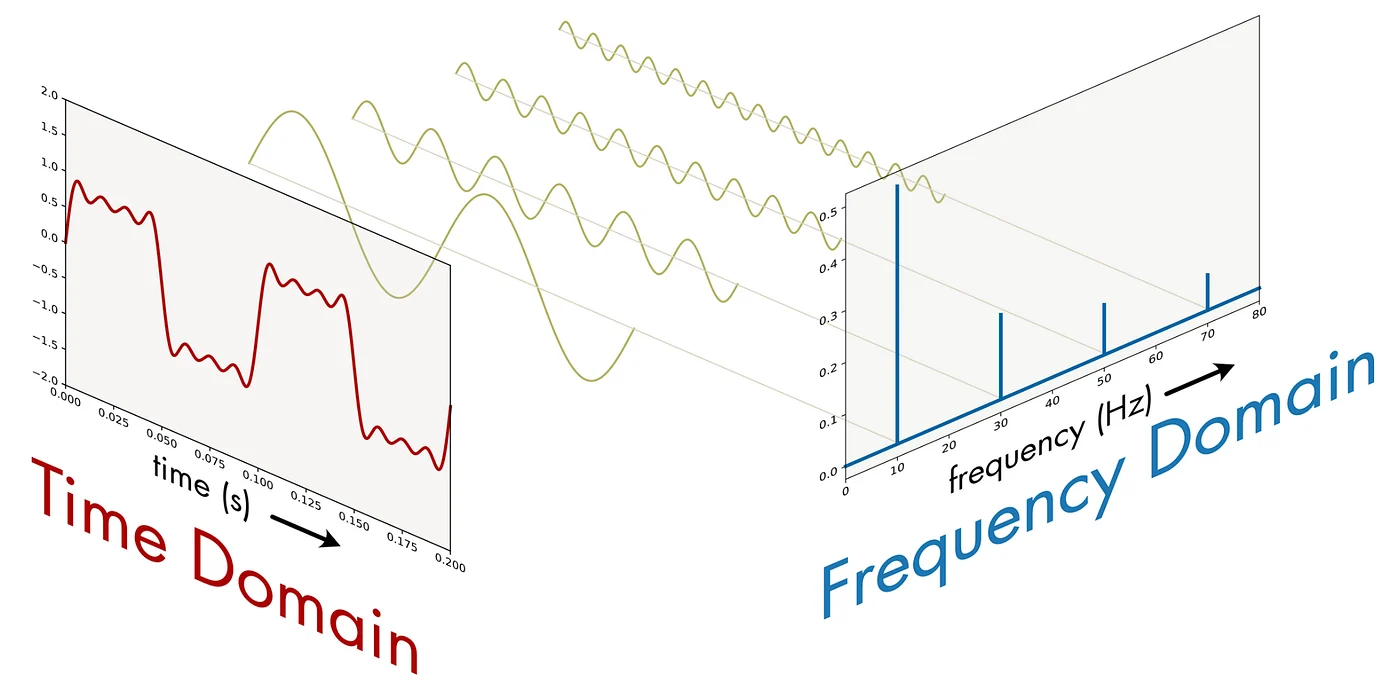A visual illustration of a signal in the time and frequency domains (Image taken from https://neurotext.library.stonybrook.edu/C7/C7_1/C7_1.html)

Time Domain

This is the framework we have used to describe speech so far. Basically, we have amplitude values (loudness) at every unit of time (a unit depends upon the sampling rate of the signal).

Frequency Domain

In contrast, the frequency domain describes a signal in the form of energy that is present at various frequencies.

Naturally, over the past decade, researchers have developed methods to perform speech recognition over the domain, separately, and together.

How Do We Solve The VRAM Issue In The Time Domain?

As we discussed earlier, CNNs were becoming increasingly popular in speech recognition before Transformers came into the picture.

Remember — Images are 2D signals, whereas audio is a 1D signal. Because convolutions can be applied to signals of any dimension, they are the perfect tool for processing waveforms.

In 2020, Facebook AI (FAIR) came out with an architecture called Wav2Vec2, which was able to learn speech representations from raw audio using CNNs. Let’s quickly understand how they solved the VRAM issue before discussing the approach in detail.

Take the raw audio and pass it through the following FeatureEncoder module,

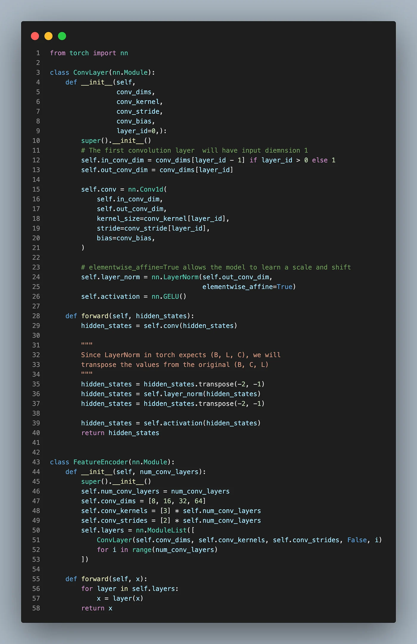A distilled version of the feature encoder used in Wav2Vec2 (Code written by the author)

Here, the ConvLayer module takes in the raw audio in the first pass (as a 1D signal) and reduces its length using stride = 2(in our case), i.e., instead of applying a convolution kernel for every single sample in our speech signal, we only apply the kernel for every other sample in our speech signal (and use the previous sample and the next sample to calculate the feature vector using a weighted summation— since kernel size = 3 in our case).
For a 3-second speech signal, we had 132300 amplitude values (from the previous section). Passing this signal through the feature encoder, we cut the number of samples in half per layer. Therefore,

132300/2⁴ = 8268.75 samples (the decimals are handled using padding to make sure that the total number of samples is always a positive integer).

This makes an attention matrix of size 8268², which is approximately 130.41 MB (WE WENT FROM 32 GB TO 130 MB BY USING JUST 4 CONVOLUTIONAL BLOCKS!!!)

In the actual Wav2Vec2 architecture, they use 7 convolutional blocks with 512 channels each, strides (5,2,2,2,2,2,2) and kernel widths (10,3,3,3,3,2,2).

Such use of convolution layers to create internal representations is popularly known as convolutional subsampling.

How Are These Latent Speech Representations Represented Using Discrete Tokens?

In language, every token is mapped to a vector in the embedding space (this mapping is used to decode tokens back from the embedding space into the token space). So theoretically, we want to achieve the following,

The latent speech representation vectors should be mapped to the closest vector in the finite set of a pre-defined “codebook”.

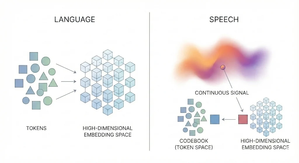The latent speech representations are vectors in a very high-dimensional embedding space, which are mapped to the closest discrete unit (Image generated using Nano Banana Pro)

This is essentially a clustering task — you have vectors in a high-dimensional space, and you want to represent them using a finite set of centroids (When the centroid IDs are used as a form of lossy compression, we call the method “Vector Quantization”). Wav2Vec2 achieves this goal by using Product Quantization with Gumbel Softmax.

Product Quantization (PQ)

We will first, quickly understand the problem with standard vector quantization. Imagine you have 128-dimensional vectors and you want to perform vector quantization, i.e., you want to map those vectors to unique IDs of 16-bit strings (say). You would need 2¹⁶ unique IDs (in case of clustering, we will call them “centroids”). The set of all the centroids is called a “codebook”. Consider Hierarchical K-Means (HKM), where you calculate a distance measure between all the centroids and club the ones that are closest together in every iteration. In this case, it’s easy to see that this is a computationally expensive operation due to the large number of centroids present in the data.

To solve this problem, Product Quantization (PQ) was proposed in 2009 with a unique insight — “Why do we want to quantize the vector into a single unique ID when we can quantize it into a smaller vector of unique IDs?” Following this principle, the author created a method where a 128-dimensional vector will be broken into m (say) distinct subvectors, and then these subvectors will be mapped to unique IDs in a subspace.

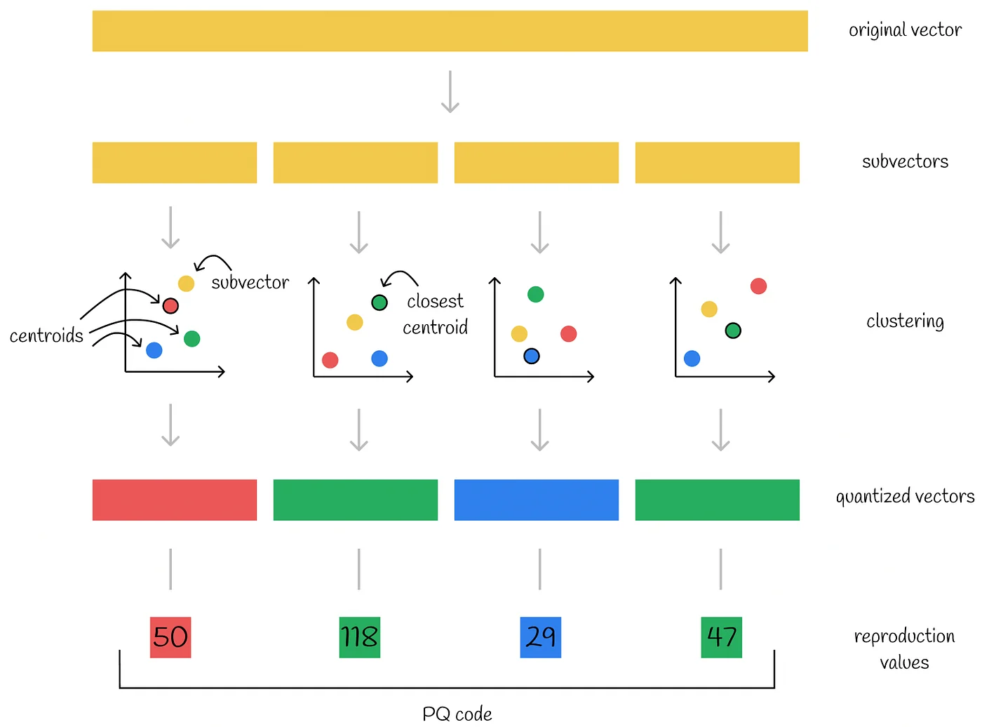The PQ code is the concatenation of the closest centroid ID for every subvector (Image taken from https://towardsdatascience.com/similarity-search-product-quantization-b2a1a6397701/)

So, following our earlier example, the 128-dimensional vector is now broken down into 8 vectors of dimension 16. Quantizing that to 0.25 bits per element (4-bit strings), we get 2⁴ = 16 centroids per subvector.

Now, for m subvectors, m separate codebooks will be trained. During inference, for a query vector, we can search the m closest centroid vectors for every subvector of the query, concatenate them, and get our final answer.

In our case, these centroids in the codebook represent the different “units” of speech that can be used as discrete tokens.

Gumbel Softmax

Given the vector of a distance measure (say, Euclidean) between the query subvector and all the centroid subvectors, how would you find out the closest centroid? The obvious answer would be to use the argmin function or the argmax of the negative vector. While this would give the correct output, there are two issues with this approach,

Gradient Discontinuity

The argmax function is a step function, meaning that it can not be differentiated (the gradients are zero everywhere except at the maximum value, where they are infinite).

2. The Problem of Codebook Collapse

If we always pick the absolute closest centroid (deterministic argmax), the model might get ‘stuck’ using only a handful of easy-to-reach centroids early in training. The other centroids never get chosen, receive no gradients, and essentially die. By sampling instead of just maximizing, we encourage the model to explore and utilize the full codebook.

So what we need is: a differentiable function that can sample from a given distribution.

Solving the first problem is fairly easy. In order to convert an argmax function into a differentiable function, we can simply replace it with a softmax function with temperature less than 1, as described below.

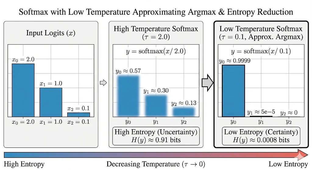When the temperature is low, softmax pushes the larger values exponentially towards infinity, which results in an approximation of the argmax function (Image generated by Nano Banana Pro)

However, this function will still always choose the centroid closest to the query vector. We need to find a way to sample from the distribution of distances using our softmax function with temperature.

This is where the Gumbel distribution comes in. Turns out, if you sample a uniform distribution between 0 and 1, perform Inverse Transform Sampling with the CDF of the Gumbel distribution, and add that to the logits (unnormalized raw scores), the softmax (with temperature) on those logits will follow the probability distribution defined by the softmax of the logits. This is called the Gumbel-Softmax Trick.

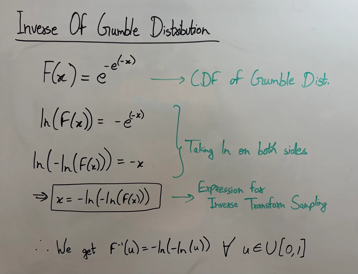Finding the inverse CDF of gumble distribution (Image clicked by author)

Inverse Transform Sampling is the method of generating any distribution by plugging in random values sampled from the standard uniform distribution into the inverse CDF of the desired distribution.

Goal: Avoid codebook collapse.

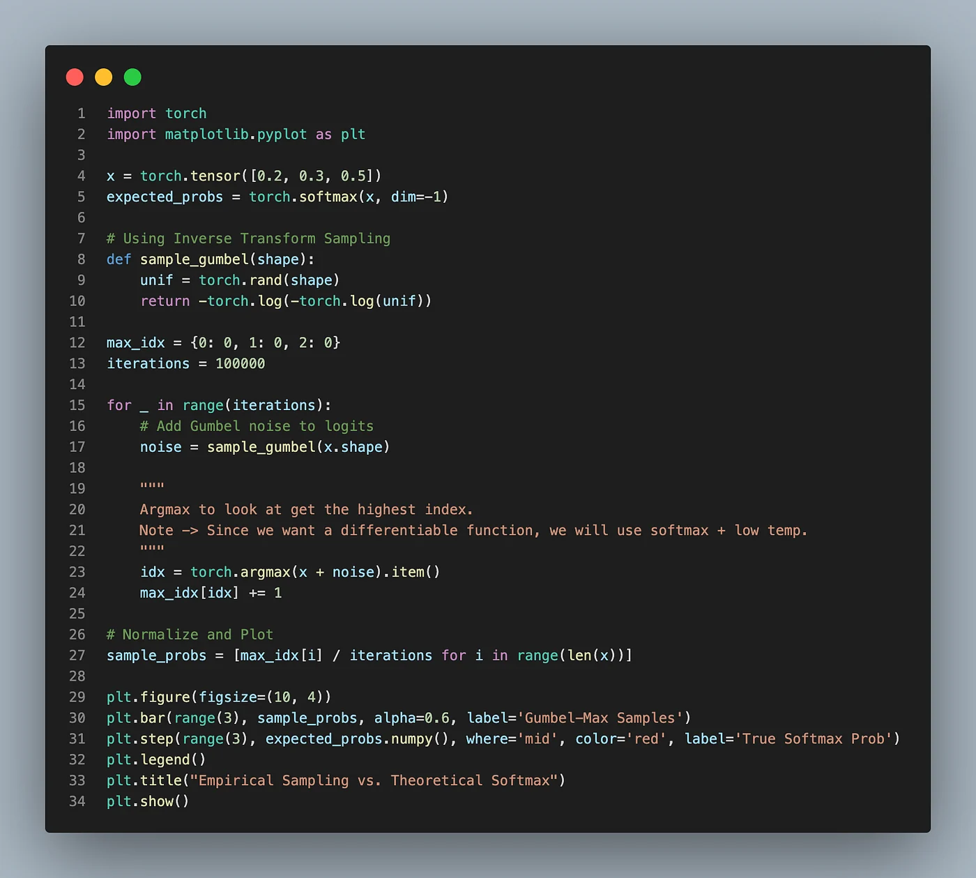We simply plot the probabilities w/o gumble noise and with gumble noise (Code written by the author)

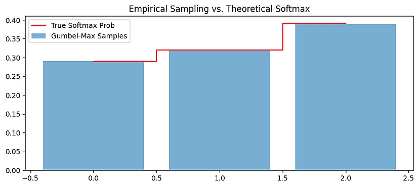The probabilities are almost identical (Plot generated by the above code)

Therefore, using the Gumbel-Softmax trick helps us achieve sampling while having a differentiable function, which means that we will avoid the problem of codebook collapse and gradient discontinuity.

The Gumbel-Softmax trick gives us the best of both worlds:

Forward Pass: It behaves like a discrete sample (picking one centroid).
Backward Pass: It allows gradients to flow through the ‘soft’ probability distribution, making the whole system differentiable.

We now have a self-supervised approach for generating discrete tokens from latent speech representations, which leaves us with a finite set of quantized representations (which the paper denotes by Q ).

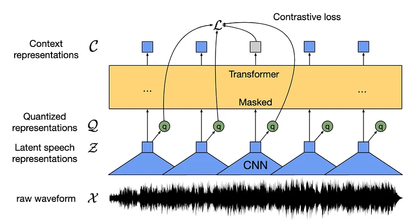Illustration of the Wav2Vec2 architecture (Image taken from the paper)

Since we are assuming the reader knows the ins and outs of the transformer architecture, let’s focus on the objective function before wrapping up our discussion in the time domain.

How Is The Transformer Trained To Understand These Discrete Units?

Taking a page from the BERT architecture, Wav2Vec2 masks some random timesteps, and the transformer’s job is to pick the correct quantized latent speech representation from a set of K representations. This set of “distractors” is uniformly sampled from the set of all masked timesteps of the same utterance.

Naturally, you would think that a similarity metric like cosine similarity will help us find the “correct” timestamp, and you would be right on the money! The loss is then the scaled cosine similarity (scaled by a hyperparameter) normalized by the sum of all the scaled similarities.

D is the set of distractors (LaTeX written by author)

Remember, the negative sign is there because we always want to minimize the loss and similarity is something we want to maximize.

For numerical stability, the authors use the LSE trick in the paper.

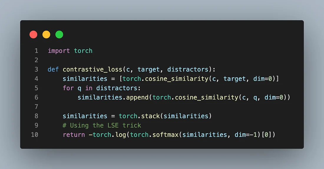Code for calculating the contrastive loss (Code written by the author)

Now, in addition to this contrastive loss, we also want to penalize the model if it keeps picking the same codebook entries again and again. The goal is to push the distribution of picking the different codebook entries towards a uniform distribution so we want to maximize the entropy of the averaged softmax distribution over the codebook entries. The authors call this the diversity loss.

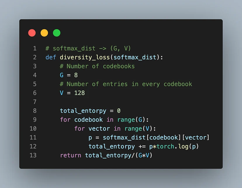Code for calculating the diversity loss (Code written by the author)

Therefore, the final objective function is the sum of contrastive loss and scaled diversity loss.

Final objective function of Wav2Vec2 in pre-training (LaTeX written by the author)

We have spent a lot of time discussing how to “brute force” our way through 1D raw waveforms using CNNs and clever loss functions. But what if we didn’t have to look at the signal as a series of amplitude points?

How Do We Solve The VRAM Issue In The Frequency Domain?

We have all done the “glass prism” experiment in high school, where white light gets separated into a continuous spectrum of colors (a rainbow) by simply passing through a glass prism. For audio signals, this “glass prism” is the Fourier transform.

When you perform a Fourier transform over an audio signal, you get the energy levels corresponding to every frequency level (e.g., 100Hz, 500Hz, 2000Hz) for the whole signal. However, when it comes to speech, taking the Fourier transform of the entire signal does not make sense as we are interested in the frequencies corresponding to every word separately and not as a single file. This leads us to Short-Time Fourier Transform (STFT) where we perform a Fourier transform over a short sliding window.

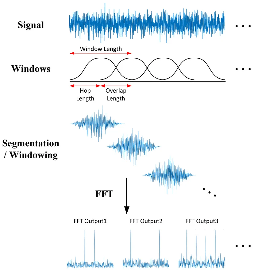Visual representation of STFT (Image taken from https://www.researchgate.net/figure/Short-time-Fourier-transform-STFT-overview_fig1_346243843)

Since these small windows all have frequency amplitudes for the same finite set of timesteps, STFT leads us to a unique representation of the speech signal where the x-axis represents the timesteps, the y-axis represents the bins of frequencies, and the color represents the energy for every time-step among all the different frequencies. This representation is popularly known as a Spectrogram.

Problem — Computers hear “linearly”, i.e., a difference between 100Hz and 200Hz is the same as the difference between 1000Hz and 1100Hz. However, humans are much better at discriminating between low frequencies than they are at discriminating between high frequencies, i.e, the difference between 100Hz and 110 Hz is very evident to a human, however, the difference between 1000Hz and 1010Hz is hardly distinguishable. This scale that mimics human hearing is known as the Mel Scale.

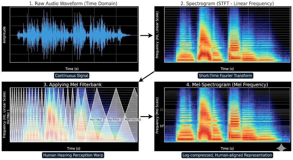Going from raw audio to a mel-spectrogram (Image generated by Nano Banana Pro)

For anyone who wants to understand the Mel-Spectrogram in more detail, I highly suggest going through this blog post.

Let’s look at the impact of this on the VRAM usage now. If we have a window of 25ms, and we slide that window 10ms in every iteration (since windows are overlapping), we get a total of 100 frames per second.

Therefore, for a 3-second audio,

\[3 \times 100 = 300 \text{ vectors}\]

Therefore, the size of our attention matrix becomes (300)², which is approximately 0.17 MB. By switching to the frequency domain, we reduce the size of the attention matrix by a factor of ~47x!

Now we’ll look at one of the most influential models of ASR history — Whisper by OpenAI. In 2022, OpenAI released the Whisper model, trained on 680,000 hours of multilingual data, and it made waves in the AI community. The architecture was nothing new, but the quality of the training data made it a huge success. Let’s quickly go over the model to understand how the ASR task works in the frequency domain.

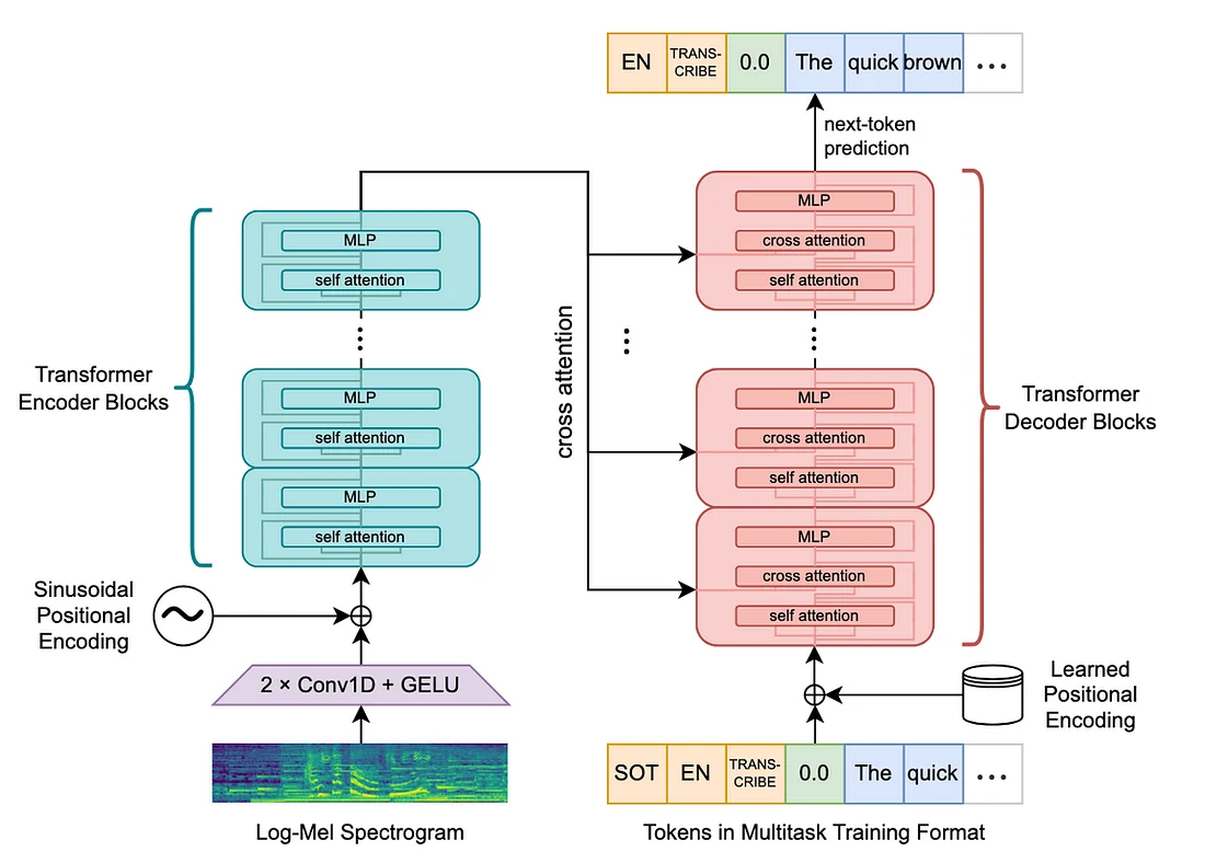Illustration of the Whisper model (Image taken from the official paper)

In the diagram above, you can see that Whisper also uses Convolutional Subsampling on top of operating in the frequency domain, which means that there are additional savings in VRAM usage.

One clear distinction from the Wav2Vec2 model is that Whisper’s training paradigm is supervised in nature instead of being self-supervised.

Since Whisper uses a standard Transformer architecture, we won’t retread old ground. Instead, the real genius of Whisper lies in how it structures its inputs and outputs to handle multiple tasks at once.

While Whisper is still one of the most dominant models in the field of ASR, the architecture of the model has not significantly pushed any boundaries in the field.

Other Significant Approaches In ASR

While Transformers are great at global attention, choosing the Transformer architecture for ASR means letting go of the inductive biases that we would be getting as a bonus if we were to use CNNs instead. Building on this idea, Google came out with an interesting approach — Conformer.

Conformer (Convolution + Transformer)

The most important inductive bias that comes with CNN (for our use case) is locality — the ability of convolutional networks to represent the local relations in a signal. To get the best of both worlds, Google came up with a transformer encoder that included a convolutional block in the Conformer paper.

Let’s quickly go over the big ideas from the paper,

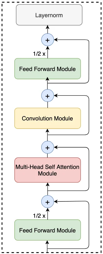Conformer Block as discussed in the official paper (Image taken from the paper)

Macaron FFN

Inspired by Macaron-Net, the Conformer paper also breaks the FFN layer in the encoder into two “half-layers”. The idea is to simply pre-process the input before it goes into the attention layer, and then post-process it, all of this, while keeping the “strength” of the signal the same as it would have been if we used the standard MHSA -> FFN.

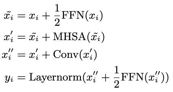We divide the output of the FFN layers in the residual connection to maintain stability (LaTeX written by author)

This helps the model reach convergence faster and gives a nice theoretical edge towards understanding the exact function that the FFN executes.

Convolution Module

Inside the encoder block, after we apply the MHSA, instead of directly processing the hidden states with a linear layer, the Conformer paper uses a convolution module to extract the local context before processing the hidden states.

Convolution Module used in the Conformer paper (Image taken from the official paper)

Inside the module, the attention scores for all the pixels in the mel-spectrogram pass through both Depthwise Convolution layers — layers that process the input using the neighbours from a single channel, and Pointwise Convolution layers — layers that process the input using a stack of pixel values (from the same coordinates) across all the channels. This helps the model in capturing fine-grained local acoustic patterns.

Neural Transducers

When RNNs and LSTMs came to play with temporal data, one big problem with using these models in speech recognition was that they were Sequence-to-Sequence models, which means that they only produced an output after the entire sequence was processed. However, speech recognition turned out to be an “online” task at times, i.e., it requires immediate outputs.

Then, in 2015, Google Brain came out with their neural transducers, which were decoders that process the encoder output for every time step and generate zero or more outputs.

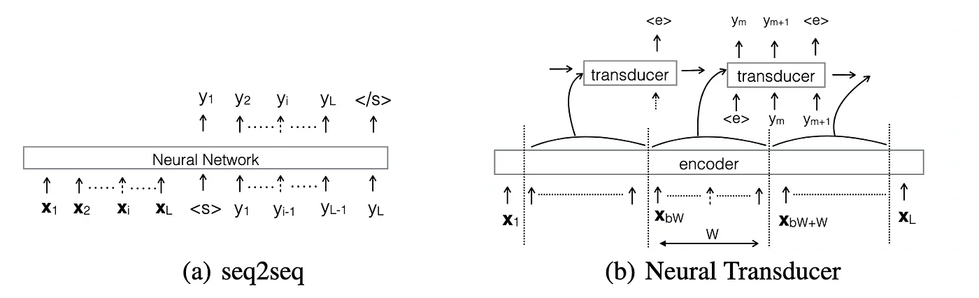Neural Transducer as introduced by Google Brain (Image taken from the official paper)

But how does it actually do that? The magic lies in a special token called the “Blank” symbol. In a standard model, every input frame forces an output. But in a Transducer, the model has a choice at every millisecond: Emit a token if it is confident or Emit a “Blank” token — This essentially means “I’m listening, but there is no new information yet,” or “I’m just waiting for the next sound.”

This architecture is the industry standard for Streaming ASR. When you talk to Siri or Google Assistant and see the words appear one by one as you speak, that is likely a Neural Transducer working in the background. Since the topic is theoretically dense and we have already covered a lot of ground, we will leave it for another article.

Starting with the raw audio, we’ve seen how “simple” math tricks like Product Quantization and the Fourier Transform save us gigabytes of memory and allow machines to truly understand human speech.

Today’s ASR systems are an engineering marvel sitting at the intersection of mathematics, statistics, physics, and computer science. While you can certainly use these models without knowing how a Mel-Filterbank works, it’s always better to be curious about the theoretical underpinnings while creating any application in order to make it more optimized.

References

1 — Baevski A, Zhou Y, Mohamed A, Auli M. wav2vec 2.0: A framework for self-supervised learning of speech representations. arXiv. Preprint posted online June 20, 2020. https://arxiv.org/abs/2006.11477

2 — Jégou H, Douze M, Schmid C. Product quantization for nearest neighbor search. IEEE Trans Pattern Anal Mach Intell. 2011;33(1):117–128. doi:10.1109/TPAMI.2010.57

3 — Jang E, Gu S, Poole B. Categorical reparameterization with Gumbel-softmax. arXiv. Preprint posted online November 3, 2016. Updated August 5, 2017. https://arxiv.org/abs/1611.01144

4 — Radford A, Kim JW, Xu T, Brockman G, McLeavey C, Sutskever I. Robust speech recognition via large-scale weak supervision. arXiv. Preprint posted online December 6, 2022. https://arxiv.org/abs/2212.04356

5 — Gulati A, Qin J, Chiu CC, et al. Conformer: convolution-augmented transformer for speech recognition. arXiv. Preprint posted online May 16, 2020. https://arxiv.org/abs/2005.08100

6 — Lu Y, Li Z, He D, et al. Understanding and improving transformer from a multi-particle dynamic system point of view. arXiv. Preprint posted online June 6, 2019. https://arxiv.org/abs/1906.02762

7 — Yu F, Koltun V. Multi-scale context aggregation by dilated convolutions. arXiv. Preprint posted online November 15, 2015. Updated April 30, 2016. https://arxiv.org/abs/1511.04868