The Biggest Enemy of Generative Modeling
“Ever heard your grandma talk about generative models?” — WHAT A STUPID QUESTION, RIGHT? Well, as it turns out, it is not a stupid question. The idea of generative models can be dated as far back as 1763 when Thomas Bayes gave the world the “Bayesian Inference”. However, this explanation only works for those of you who look at generative modeling as a task in Bayesian statistics.
For the frequentist approach, the earliest work in generative modeling can be traced back approximately to the 1920s when Ronald Fisher connected Maximum Likelihood Estimation (MLE) to statistical modeling. Here, we take both views into account and understand how today’s scientists have successfully evaded the evils of approximating an underlying distribution. Before going ahead, let us finalize some notations for the entire article.
\(\{x^{n}\}_{n=1}^{N} - \text{Observed data samples}\) \(p_\theta(x) - \text{Arbitrary model family parameterized by }\theta\) \(q_{data}(x) - \text{"True but unknown" data distribution}\) \(p(z|x) - \text{Conditional probabiltiy distribution of z given x}\)
But What Is This “Evil”?
In the axioms of probability, the probability distributions must sum up to 1 in order to be valid.
\[\int{p(x)}dx = 1\]The problem of generative modeling, in its most abstract form, is simply a problem of approximating a probability distribution to the true data distribution.
\[p_\theta(x) \approx q_{data}(x)\]However, the probability distribution in question is usually approximated using neural networks (which try to fit flexible functions into the existing data). These functions are always learned in their unnormalized forms unless defined explicitly (like the softmax layer in the transformer paper). This is where the problem arises — to sample from a probability distribution, we need it to be normalized. Why?
Sampling essentially means picking out data points from a distribution with the following constraint on the amount of data that can lie in a particular area (A),
\[p(x\in A) = \int_{A}{p(x)}dx\]But when the distribution is unnormalized, sampling takes the following form,
\[p(x\in A) = \frac{\int_{A}{f(x)}dxA}{\int{f(x)}dx}\]where $f(x)$ is the function represented by the neural network (unnormalized function).
This introduces a normalization constant in our equation that is computationally intractable when we have functions that have millions of parameters, since you can not compute it in its closed form. Therefore, the “evil” here is this intractable integral without which we fail to sample new data points from our underlying distribution.
Now that we have understood the evil at hand, we will look at all the major classes of generative models and see how exactly they evaded this evil.
Variational Autoencoders (VAEs)
Problem at hand — “How can we perform efficient approximate inference and learning with directed probabilistic models whose continuous latent variables and/or parameters have intractable posterior distributions?” (p.s. this is the first line of the VAE paper)
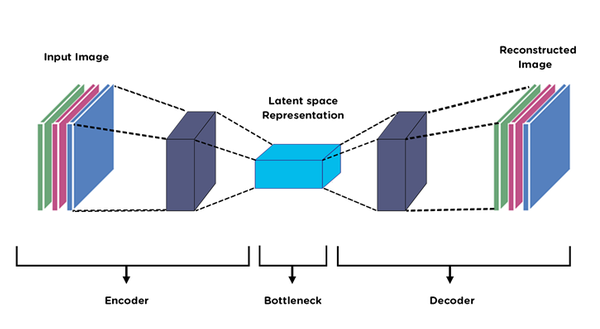
The autoencoder model circles around the existence of latent variables — variables that define the inputs but are not directly observed.
\(p(x, z) = p(z).p(x|z)\)
Therefore, our goal becomes to model the following marginal likelihood,
\[p(x) = \int{p(z)p(x|z)dz}\]The prior p(z) is designed to be tractable (usually a multivariate standard normal distribution). However, this marginal becomes intractable due to the following reasons:
p(x|z)is non-linear (since it is a neural network — decoder).zusually has a very high dimension.- there is no closed-form solution to the integral.
Note — Before coming to p(x|z) i.e., the decoder, we have to talk about p(z|x), i.e., the encoder, which faces the same problem of intractability.
Continuing with our task of avoiding the integral, we use the oldest trick in the book and introduce a variational distribution (i.e., the encoder),
\[p(x) = \int{\frac{p(x, z)}{q(z|x)}.q(z|x)}\]Let us recollect what we know about KL-Divergence,
\[D_{KL}[q(z|x)||p(z|x)] = \mathbb{E}_{q(z|x)}[\log{\frac{q(z|x)}{p(z|x)}}]\]Using Bayes’ Rule,
\[p(z|x) = \frac{p(x, z)}{p(x)}\]The earlier equation becomes,
\[D_{KL}[q(z|x)||p(z|x)] = \mathbb{E}_{q(z|x)}[\log{\frac{q(z|x)}{p(x, z)}} + \log{p(x)}]\]Since $p(x)$ is a constant w.r.t $z$, we get,
\[\log{p(x)} = D_{KL}[q(z|x)||p(z|x)] + \mathbb{E}_{q(z|x)}[\log{\frac{p(x, z)}{q(z|x)}}]\]The expectation part is what we call the lower bound on the marginal likelihood of the observed data.
Okay, perfect! Now, since KL Divergence is always non-negative, we can drop that from the above equation to formulate the following inequality:
\[\log{p(x)} \geq \mathbb{E}_{q(z|x)}[\log{p(x|z)}] - D_{KL}[q(z|x)||p(z)]\]The RHS here is known as the Evidence Lower Bound (ELBO). The main objective of a VAE is to maximize ELBO (which doesn’t require any knowledge about p(x) and the KL Divergence is often analytically calculated as the prior distribution is chosen to be a standard normal distribution).
Furthermore, the reparameterization trick is used to optimize the parameters by using the standard gradient methods.
Therefore, by maximizing ELBO and using the reparameterization trick, VAEs dodge the “evil” of the intractable integral and are able to learn from the data and later provide inference on it.
Generative Adversarial Networks (GANs)
Unlike VAEs, GANs avoid the intractable integral by removing the need for probability densities altogether.
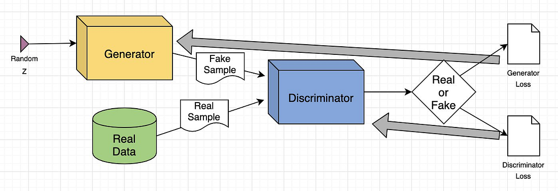 An overview of the architecture of GAN architecture (Image taken from
this link)
An overview of the architecture of GAN architecture (Image taken from
this link)
Here’s a quick intro about how a GAN learns,
The generator (`G`) takes in a random noise vector (`z`) and tries to mimic the real distribution by mapping the noise vector to a data space, `x=G(z)`. Then, the discriminator (`D`) takes in that output and generates a probability score indicating whether or not the input came from the real dataset. Both, the generator and the discriminator keep trying to outsmart eachother and as a result, learn the data distribution IMPLICITLY.
Now, let us look into how this happens mathematically. For those of you familiar with game theory, the learning process of a GAN is simply a two-player zero-sum game. Simply put, this means that the game is devised in such a way that one player’s profit is directly proportional to the other player’s loss.
So, here V is trying to maximize the payoff function to identify more samples correctly and G is trying to minimize the payoff function to fool the discriminator.
Okay, now you can ask, “Cool! But how long does it keep playing the game?”. Well, there is a concept in game theory called “Nash Equilibrium,” which is basically a state in which neither player can improve its payoff without the other player changing its state (parameters, in our case). This is the “ideal” state for a GAN to be in at the end of its training. When a GAN is in equilibrium, the following two conditions are true,
1 — The generator (G) samples from the real distribution of the data.
2 — The discriminator (D) is unable to distinguish the fake samples from the real ones, i.e.,
However, in practice, this type of convergence is seldom seen due to,
- Non-convexity of the optimization plane
- Optimization instability
Therefore, we see that Ian Goodfellow created GANs as a completely new set of generative models that approximate the densities in an implicit fashion. Although vanilla GANs had training issues, the variants also follow the same underlying structure that we talked about, except for some changes to the loss function.
Note -> GANs are strictly non-Bayesian in nature.
Energy-Based Models (EBMs)
An energy-based model defines the probability of a data point x using an unnormalized density:
This clearly translates to the “evil” that we are trying to evade, i.e., Z(\theta) — the normalization constant is an intractable integral.
The only difference here is that we have an “energy function” — E(\theta) ; but why is that? Anyone who has studied a semester of statistical physics would instantly recognize the above equation as a special case of the Boltzmann distribution (with kT = 1) — a distribution in thermodynamics that describes the probability of a system being in the state x.
The whole idea is to look at a system as an energy landscape with the energy at any particular state defining the probability of the system to be present in that state. Higher the energy of a state, lower the probability of the system to be in that state.
 Model learning the low energy regions (Animation taken from
Michal’s corner)
Model learning the low energy regions (Animation taken from
Michal’s corner)
This works well with our understanding of the optimization plane — reach the minima if you want to learn the patterns in the training data. Here, the valleys correspond to the training data, and the hills correspond to irrelevant regions.
Got it! But how do EBMs evade the curse of the normalization factor?
Over the years, different approaches have been developed to train EBMs without having to deal with the intractable integral. Here, we will only discuss one approach in depth.
Score Matching
The idea is to eliminate the intractable integral by calculating the gradient of the log likelihood with respect to x (remember, in MLE, this gradient would have been w.r.t the parameters — \theta)
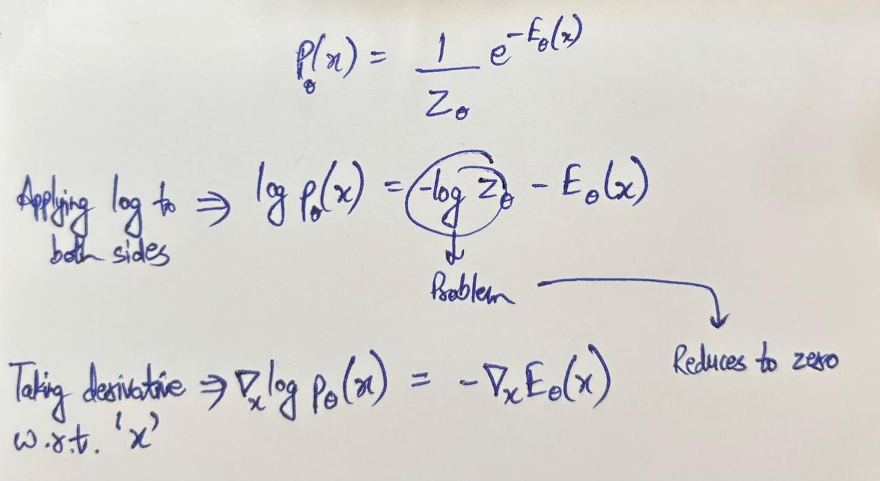 This gradient of the log likelihood is also known as the **score function**
Score matching then optimizes the Fisher Divergence to minimize the difference between the model distribution and the true distribution,
\[\mathbb{E}_{q_{data}}[\| \nabla_x \log p_\theta(x) - \nabla_x \log q_{data}(x) \|^2]\]Now you might be wondering that “Okay, we got rid of the intractable integral, but the second term in the absolute expression is still intractable as we only know the observed data points,” AND YOU’D BE RIGHT!
We won’t go through the whole thing here, but by using integration by parts and an assumption that densities at infinity can be ignored, the above function gets reduced to this:
As you can see, now there is absolutely no dependency on any intractable term, and we can start training our model by optimizing the above function!
Note —> Other techniques to avoid the normalization constant also exist, mainly “Contrastive Divergence” and “Noise Contrastive Elimination,” but that is beyond the scope of this article.
EBMs give a nice geometric meaning to the functions being modeled by our neural networks and have therefore found an audience in niche fields.
Flow-Based Models
Taking a very bold approach and facing the problem head-on, NFs don’t avoid the intractable integral — THEY MAKE IT TRACTABLE!
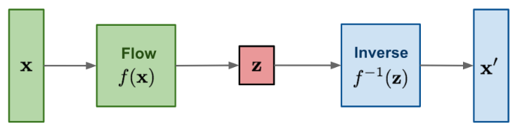 General architecture of a flow-based generative model (Image taken from
Lilian Weng’s blog)
General architecture of a flow-based generative model (Image taken from
Lilian Weng’s blog)
Flow-based models use what is known as a “Normalizing Flow,” which, simply put, is a bijective, differentiable, and invertible transformation:
\[x = f_{\theta}(z), z = f^{-1}_{\theta}(x)\]Using the change-of-variables formula, we get the probability induced on x by this transformation:
The Jacobian of the inverse is difficult to find (computationally), therefore, we will apply a log transformation to the above equation, resulting in the exact log-likelihood, which is also computationally computable if the following conditions are met,
- The inverse of the transformation is tractable.
- The Jacobian determinant is tractable.
That sounds pretty neat! But how can a neural network make sure these conditions are met?
Flows are typically not complex at all — they are composed of many simple invertible transformations,
\[f_\theta = f_K \circ f_{K-1} \circ \cdots \circ f_1\]This architectural constraint is the main reason why flow-based models are so complex and are generally not preferred.
Diffusion Models
This is the final class of models we will look at, and it is the most interesting one of them all. Diffusion models employ a two-step strategy to evade the problem of the normalization constant.
Note -> We won’t go into the depths of each component in the diffusion model, as that is a tangent that truly deserves its own post. We will only look at the model, trying to find that normalization constant and eliminating it.
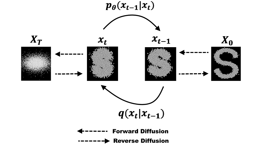 Diffusion models have a forward process and a reverse process (Image taken from
this blog)
Diffusion models have a forward process and a reverse process (Image taken from
this blog)
1 - Forward Process
The input to the forward process is a pure image, and the intended output is pure noise. This conversion takes T timesteps (say), and at every step, noise is sampled from a Gaussian distribution and added to the image,
However, since this is a predictable process (Gaussian throughout) that follows closed-form sampling, we don’t need to do this iteratively. We can just use the following expression to calculate what the image will look like at any given timestep,
So, the forward process doesn’t deal with the normalization constant at all.
2 — Reverse Process
The reverse process aims to go back to the original image, one step at a time,
\[p_{\theta}(x_{t-1}|x_{t})\]However, since this value is intractable, a clever way to avoid this is to train a network that calculates how much noise was added to the image at this step using a “denoising” score matching objective.
This score matching works exactly like how we saw in the case of Energy-Based Models (EBMs), with an added twist of corrupted inputs and known conditionals (how the corrupted inputs were made from the original image).
Therefore, the score matching directly tells the model “which is the steepest way to go upwards”. Following this strategy, we get a neural network in the end that is able to approximate the score for each noise level.
By this point, it should be clear that diffusion models avoid dealing with the data distribution at all by making a neural network do all the heavy lifting with an objective inspired by the Fisher Divergence.
Therefore, we saw that different types of models deal with this “evil” in different ways. There is no “correct” way, but the problem can always be looked at from different angles, and there is always room for improvement.
Note -> Autoregressive models are a class that we did not talk about, but that is because they have an inbuilt normalization factor that makes sure that all the conditionals in the joint probability are normalized beforehand. This enables them to perform exact evaluations of the log-likelihood.
References
3 - VAE Paper
4 - GAN Paper
6 - Jake Tae’s Blog
7 - Lilian Weng’s Blog on VAEs
8 - HuggingFace’s Blog on Diffusion
9 - Lilian Weng’s Blog on EBMs
10 - Michal’s Corner