Transformer²: The Death of LoRA?
The idea behind sakana.ai’s latest research paper, which provides a general framework for a new type of transformer architecture, is that of adaptation. Much like your toxic partner who turns into a sweetheart as soon as external observers are available, LLMs need to adapt to a wide variety of tasks to be suitable for domain-specific usage.
 Photo by Cécile Brasseur on Unsplash
However, traditional LLM post-training has several downsides,
- Fine-tuning is highly resource intensive — Even with modern techniques like the usage of mixed precision, quantization, and PEFT, the process of fine-tuning an LLM is still expensive and demands both computation and storage.
- Overfitting Issues — More often than not, the fine-tuned model starts generating repetitive outputs and is doomed for catastrophic forgetting.
- Task Interference — Conflicting gradients usually result in the model performing better at one particular task while suffering a degradation in the performance of another task.
Self-Adaptive LLMs
We define self-adaptive LLMs as a class of models that have the ability to regulate its behaviour with respect to dynamic changes in the environment without any external interference.
How can we achieve such intelligent models?
-
Improving existing LLMs — We are all familiar with the scaling laws and emergent capabilities of LLMs, so it should not come as a surprise that if we keep creating bigger models, they will obviously be better at performing a wide variety of tasks with decent outputs across multiple domains. However, this is not a very scalable idea and needs immense computing power.
-
Using Mixture-Of-Experts — MoE is the idea of dynamically routing the inputs to “expert” modules that specialize in a specific domain. The authors suggest that Transformer² can be loosely categorized as an MoE model but differs in significant ways.
Last year, a paper titled “Self-MoE: Towards Compositional Large Language Models With Self-Specialized Experts” came out of MIT and Georgia Tech that introduced an approach to convert monolithic LLMs into compositional systems. The idea is — instead of human-labeled data (like in the case of MoE), individual expert modules are created from scratch using synthetic data. These modules are then shared by the base LLM, which routes specific inputs to a particular module.
Benefits of Self-Adaptive LLMs,
- Dynamic modification of the model for different tasks without the need for fine-tuning again and again.
- Continual Learning — Over time, the model can accumulate information instead of being trained with static information.
- Eliminating Catastrophic Forgetting — New information can be added to the model without triggering any form of catastrophic forgetting, where the model forgets how to do a previous task after learning a new task.
The authors also highlight the fact that self-adaptive LLMs mimic the neuroscientific principle of “activating specific areas of the brain depending upon the task at hand”.
While MoEs are a great way to create compositional systems, training a separate “expert” module for each individual task is still a resource-intensive approach. To tackle this issue, the paper introduces a novel technique for fine-tuning — Singular Value Fine-Tuning (SVF).
Singular Value Fine-Tuning
Before jumping into the technique used by the authors of the paper, let us take a look at some of the fundamental concepts required to understand this methodology.
Fine-tuning with Singular Value Decomposition (SVD)
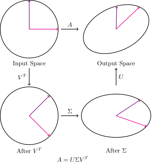
In SVD, both U and V rotate the vector space. Our subject of interest here is the Σ matrix.
Note that when Σ scales the vectors by their corresponding singular values, the basis vectors are aligned with the principal axes (direction of maximum variance). Therefore, changing the scaling values can be looked at as changing the amount of weightage that we are giving any particular principal axis.
Since these singular values can approximate the “importance” of different “features,” we can neglect the changes in V and U.
Therefore, we only update the singular values of the weight matrices while fine-tuning a network, which results in an exponential decrease in the number of parameters that need to be trained.
The only drawback of this approach is that when we train only the top-k singular values, there might be some information loss (depending on how uniform the variance is in different directions).
Comparison of SVD based Fine-tuning with LoRA
Loading the model,
from transformers import AutoModelForCausalLM, AutoTokenizer

name = "Qwen/Qwen2.5-1.5B-Instruct"
model = AutoModelForCausalLM.from_pretrained(name)
tokenizer = AutoTokenizer.from_pretrained(name)
Looking at the number of trainable parameters when using LoRA,
from peft import LoraConfig, peft_model

lora_config = LoraConfig(
    task_type="CAUSAL_LM",
    r=8,
    lora_alpha=32,
    lora_dropout=0.1,
    bias="none",
)

lora_model = peft_model.get_peft_model(model, lora_config)
lora_model.print_trainable_parameters()

Looking at the number of trainable parameters when using SVD (Updating all the 3 matrices — U, V, and Σ),
# SVD
from svd_training.svd_model import SVDForCausalLM

svd_model = SVDForCausalLM.create_from_model(model, rank_fraction=0.1)
print(f"trainable params: {svd_model.num_parameters(only_trainable=True)} || all params: {svd_model.num_parameters()} || trainable%: {svd_model.num_parameters(only_trainable=True) / svd_model.num_parameters()}")

Clearly, the number of trainable parameters is more when using SVD based fine-tuning, but why? Well the answer lies in the fact that we are not just updating the singular values but ALL the values in the decomposed matrices.
Following is what the model looks like after appplying SVD decomposition,
Qwen2ForCausalLM(
  (model): Qwen2Model(
    (embed_tokens): Embedding(151936, 1536)
    (layers): ModuleList(
      (0-27): 28 x Qwen2DecoderLayer(
        (self_attn): Qwen2SdpaAttention(
          (q_proj): SVDLinear()
          (k_proj): SVDLinear()
          (v_proj): SVDLinear()
          (o_proj): SVDLinear()
          (rotary_emb): Qwen2RotaryEmbedding()
        )
        (mlp): Qwen2MLP(
          (gate_proj): SVDLinear()
          (up_proj): SVDLinear()
          (down_proj): SVDLinear()
          (act_fn): SiLU()
        )
        (input_layernorm): Qwen2RMSNorm()
        (post_attention_layernorm): Qwen2RMSNorm()
      )
    )
    (norm): Qwen2RMSNorm()
  )
  (lm_head): SVDLinear()
)
Let us do some computation. There are 28 decoder layers and every decoder layer has 7 SVD linear layers. In addition, there is a model head that has also been converted to an SVD Linear layer. Therefore, we have,
\[28 * 7 + 1 = 197 \text{ SVD Linear Layers}\]Keeping everything frozen except the singular values in the Σ matrix, we have 1536 singular values per SVD linear layer. Therefore, the total number of singular values become,
\[1536 * 197 = 302,592 \text{ singular values}\]This is the effective number of parameters that will be trained in Singular Value Fine-Tuning, which equates to 0.00129% of the number of parameters being used by LoRA.
Similar work was done in the LoRA-XS paper that came out last year. However, this work introduces reinforcement learning to enhance learning efficiency.
Coming to the most important contribution of the paper: Transformer²
The framework has been broken down into 2 key steps,
- Using SVF to learn RL compact and compositional expert vectors based on the SVD of the base model’s weights. (Left in the image below)
- 3 adaption strategies that combine the expert vectors during inference. (Right in the image below)
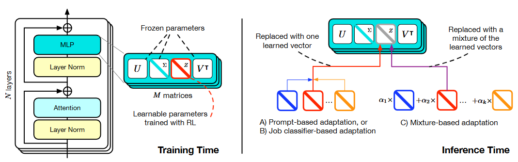 Overview of the method used in the paper (Image provided in the paper)
We looked at extensive code to understand SVF ealier in this post. Let us now look at how these expert vectors are trained with RL. We previously understood that only the Σ matrix needs to be updated. Mathematically, we can say,

where z is the SVF expert vector.
Then, the authors in the paper use the REINFORCE algorithm with a unitary reward and a KL penalty for deviating from the original model behaviour. This approach helps in creating better “expert” vectors and relaxes the constraints on the dataset to be extensive.
One big plus that these expert vectors enjoy is the high compositionality that they provide. These vectors are highly interpretable and open to algebraic manipulation.
How does the self-adaptation part work?
The framework defines a two-pass adaptation strategy that combines K sets of base “expert” vectors.
- First inference pass — Given a task, the model’s test behaviour is observed and a z’ vector is created that encapsulates this behaviour.
- Second inference pass — This adapted vector z’ is used to generate the actual response.
The idea is that by observing the test-time behaviour, the model can adapt to include any linear combination of the expert vectors at its disposal to generate the final output.
Conclusion
While the paper definitely dicusses an innovative way of building self-adaptive LLMs, creation of expert SVF vectors is more complicated than using separate modules, like in the case of LoRA. In addition, there is huge library support for PEFT techniques which make it simpler for the end users. However, SVF is definitely worth looking into if you have a deep understanding of what your weight matrices look like and how you want to manipulate them.
The paper delivers promising results but take it with a grain of salt and decide what is best for your particular use-case as I can not provide you with a comprehensive comparision due to lack of computing power :)
Note -> Images by the author have been created using LaTeX.
References
1 — Transformer² Paper — https://arxiv.org/pdf/2501.06252
2 — Sakana Blog - https://sakana.ai/transformer-squared/
3 — Self-MoE Paper: https://arxiv.org/pdf/2406.12034
4 — LoRA-XS paper: https://arxiv.org/pdf/2405.17604
5 — Truncated SVD: https://en.wikipedia.org/wiki/Singular_value_decomposition#Truncated_SVD
6 — SVD Training: https://huggingface.co/blog/fractalego/svd-training